Analyzing Housing Prices in Berkeley

This project was done with Yika Luo and Shashank Bhargava, who are also both students at UC Berkeley.

November’s always the longest month of fall semester. The days get shorter, the afternoons get colder, rain starts falling, the leaves start falling (kidding, we don’t have autumn in California), and for Berkeley seniors, it’s the deadline for having your future figured out. Interviews, offers, negotiation - it’s like no one can talk about anything else. And, as people start getting offers, they start thinking about moving into a new city.

Being that this is Berkeley, a lot of people are moving to San Francisco after graduation, where rent prices are more expensive than organ donations (and apartments are probably harder to get than the aforementioned organs). An influx of (relatively) highly-paid tech workers along with a lack of new development has driven SF’s cost of living to unsustainably high levels, and it makes moving to the city a difficult decision.

Rising rent in San Francisco then creates upward pressure on prices throughout the Bay, as people look outside the city to find more reasonable housing. Places like Oakland, South San Francisco, and Berkeley have all seen marked increases in rent prices that parallel San Francisco’s. In particular, in Berkeley, this has had a compounding effect on already highly-demanded student-housing, increasing prices for students throughout the city. Berkeley already has a culture of off-campus housing. University housing is typically overpriced, and students move into their own apartments as early as possible. This leads to an incredibly competitive apartment search starting in March and persisting through August, which is only made worse by highly-paid engineers bidding up rents and forcing a lot of students out of traditionally student-dominated housing.

I started this project actually over the summer, when a number of my friends were looking for apartments. Back then, the idea was to create a craigslist scraper that notified you when an apartment fitting your criteria was posted. After some work though, I realized that studying rental trends themselves would be a much more interesting exercise, given that there’s a wealth of data that’s publicly available. And so, that’s what this article is: I analyze rent data from two different sources, the Berkeley Rent Collection Board, and Craigslist, and use it first to both understand the current housing situation, and second apply some basic Machine Learning to understand what features drive apartment pricing.

General Housing Trends

First, here’s a general histogram of prices in Berkeley. This is based on data collected from Berkeley’s Rent Collection Board, from which I was able to scrape rent information for 9143 currently occupied apartments in Berkeley, with leases starting from 2014. This is the price per room, averaged over the number of apartment buildings (I assumed that every building’s rent per room was very similar due to rent-control).

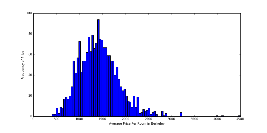
As we can clearly see, this takes on a standard, normally-distributed shape, with an average of about 1400 and a standard deviation of around 200 dollars.

But, we want to explore the relationship of prices over time, and this isn’t all that helpful in understanding that story. Instead, lets look at this histogram mapping every month to the number of leases initiated in that month:

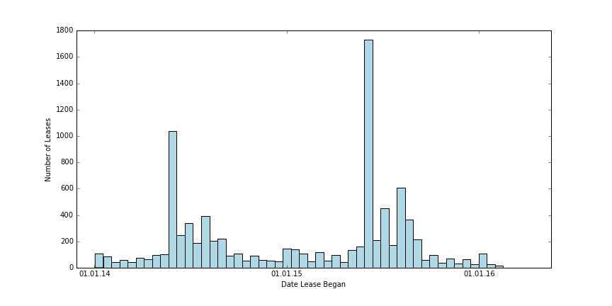
Ah, now this is more interesting. There’s clearly a spike in leases around May of every year, paralleling Berkeley’s academic calendar - school for the year ends in May, and people are finalizing their living arrangements for the next semester. This amount declines until January, when it starts rising again in the same pattern. Also, you’ll notice that the total number of leases in 2015 is clearly more than in 2014, though the pattern of buying is the same.

Then, combining the information from the two above graphs, we’d expect both a general uptick in prices over the past two years, and a rise in prices around May to August. Lets confirm that:

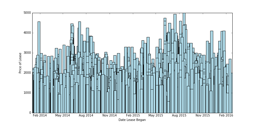
And that’s exactly what we see! Rent prices for leases starting in May are clearly higher than in November through January. And, rent prices peak in July/August of each year, which makes sense: students buying that late are desperate for apartments and are willing to pay a premium for the limited remaining supply. We can also see a general rising trend in prices from 2014 to 2016, if you compare the same month across multiple years.

Now, this gives us a general idea of rising rents across the entire city of Berkeley, with a majority of our data coming from mainly student-occupied housing. But, it doesn’t account for local variation within the city itself. To tell that story, I made this map, which gives you information on rents in Berkeley in different sectors of the city, along with a bunch of other information: distance from campus (that is, to a point that’s almost equidistant from each edge of campus), average room size (in square feet), and the average number of bedrooms. The extra information is taken by matching rent board data to Craigslist listings. There was about a 20% overlap for most sectors, so that data isn’t that representative of the region, but it serves as a useful reference point.

As you can see, there are significant differences in pricing across neighborhoods. West Side seems to be, on average, the cheapest, but it also has the smallest room size. It also has lowest average number of bedrooms, indicating a higher percentage of 1 bedroom and studio apartments than elsewhere.

Far North seems to have the largest apartments, but it has the farthest average distance to campus (it’s also a long uphill walk, ugh). South Side has also a very high average price, and it’s the closest to campus, and it’s probably the most popular region for most. North Side seems to be the most expensive, but this may be skewed by a much lower density of student housing in that area (mostly engineers live on North Side).

Finding an Intrinsic Price

Now that we have a better understanding of rent pricing in Berkeley, lets change course, and ask a more fundamental question: what is the intrinsic value of an apartment?

Economics says that all available information about an apartment is encompassed in its current price, and so, it has no intrinsic value: its value is the price people are willing to pay (this is actually also the central assumption of technical stock analysis). This definition, however, isn’t particularly useful for us now, and so, I propose a different one.

The intrinsic value of an apartment with some arbitrary feature vector is what another apartment, with exactly the same feature vector, would sell for, averaged over all other apartments (where a feature represents some quantity of the apartment that we can measure. Here, a feature could be square footage, or number of bathrooms, etc.)

But, this is the exactly the same problem as predicting prices! If we had some training set and a machine learning model trained on this training set, then, the price that model predicts for a given apartment is that apartment’s intrinsic value (what that apartment would cost if we cared only about its features). Then, we can compare the actual price of that apartment and determine whether it’s overvalued or undervalued relative to its intrinsic price.

And that’s what I did. I scraped about 1500 Craigslist listings over the past few days, parsed them, and used a Ridge Regression model to predict prices for any new listing.

Why Ridge Regression?

Why Ridge Regression? Well, the obvious reason is that it performed the best. On a 10-fold cross validation test, Ridge Regression gave an accuracy of about 42%, with a standard deviation of 22%. I also only have 7000 listings, a pretty small training set, and more complicated models will overfit on such a small set (and they did: I tried a 3-layer neural network and a random forest, both of which performed significantly worse).

But beyond that, I wanted to maintain interpretability. I’m using this model as a measure of intrinsic price, not for price prediction, and so I wanted to easily understand the amount each feature influences the final price, and ensure that the intrinsic price idea isn’t obscured by the complication of the model. For example, a neural network makes it much harder to discuss intrinsic value, because it obscures how information is combined to create predictions. A regression model, for comparison, is fairly transparent: it uses linear algebra to assign weights to each feature, and does a vector inner product to generate each prediction.

Features

My features for the model were square footage, number of bedrooms, number of bathrooms, distance from campus (that is, the distance from the closest side of a bounding box that encompasses the Berkeley campus), the number of images in the listing, the number of unique words in the description, and the number of days since the listing was posted.

What Matters Most in Determining Prices?

Here are the weights of each feature in our model:

('bedrooms', -0.01484452500338929), 
('bathrooms', 441.35475406327225), 
('square feet', 0.81243297704451789), 
('distance_to_campus', -82.126291331406136), 
('num_images', 37.305112110230304), 
('unique_words', 0.51051340095473563), 
('postingDate', 8.1268498554076096)

This means that every additional bathroom, for example, added 441 dollars to the posting price. Every square foot added about 80 cents to the price, while every additional mile from campus reduced the price by 82 dollars. This is mostly in line with what we saw in the map, before. The South Side sector is about $100 more expensive than the Far South, and it’s about 1.5 miles farther from campus, on average.

Note that the weight for bedrooms is anomalous, and it’s caused by having relatively few listings with bedrooms listed. It also comes from studios (listed as having 0 bedrooms) being high-priced and low in number in Berkeley, skewing the data. As a larger cause, this problem stems from predicting based on a very small dataset. I plan on running my scraper daily for a month using cron, and I’ll update this post once I do have more data.

And, to further expand on the relationship between distance and price, here’s another map, this one showing the average price for concentric rings radially expanding outward from campus, with all apartments within a ring roughly equidistant from campus.

As we can see, while there’s a general trend of decreasing prices, this isn’t universally true. Some outer rings are more expensive than inner rings. This is mostly due to apartments that are further from campus being larger on average, and being more likely to have more than one bathroom, which has a larger effect on price than distance does (which we saw in the weights).

So, lets say we want to find the intrinsic value of some arbitrary apartment, like this one:

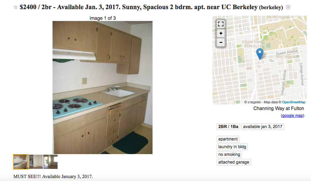
Then, if we calculate each feature, multiply it by its corresponding weight, and add it together, we get 2507.84967859 as our prediction, which is pretty close (there’s a lot of text not visible in the screenshot). Then, this listing is undervalued based upon the model’s perception of its quality, and so, we should consider renting it.

Listing-Specific Features

Lets discuss our features a bit more. The first few are obvious: bedrooms, bathrooms, square footage, and distance to campus. But the last three are a bit unique: the number of images, the number of unique words in the description, and the number of days since it’s been posted.

For every new image, the listing price increases by 37 dollars. But this makes sense: the more images you have, the more confidence you tend to have in your apartment, and so, it’s more likely your asking price will be higher (and, people with cheaper places won’t want to post pictures to show why their place is cheaper). Similarly, each word in our description adds 50 cents to the final price, which again is intuitive: a longer description indicates you believe your apartment is a highly demanded place to live, and so you’ll justify it.

Price also increases 8 dollars for every day the listing is up. But this is a product of human behavior: cheaper listings would be taken more quickly, and so only the high-priced listings stay up for longer time periods.

How to Find Undervalued Apartments

Now that we’ve articulated the idea of intrinsic price, created a model to calculate intrinsic price, and understood how and why this model behaves as it does, we can finally address the actual motivation for this post: how can we find undervalued apartments on Craigslist? Put more simply, how do we find good deals?

Well, from our analysis, we know that the age of a listing is a major component of its price. Cheaper listings seem to be taken more quickly, as we’d expect. So, be first! Check Craigslist constantly, or better, write a script to scrape Craigslist and return you interesting listings, and make sure you’re early for every listing.

And, look for the less verbose listings with fewer images. Yes, a lot of these will be terrible, but not all. In my experience, there’s a subset of listings that are for high-quality apartments being listed by people who have no idea how to sell an apartment (next project - find them?). The descriptions will be short and full of misspellings; the images will be poorly lit and unappealing. But, the price will be lower, and the apartment itself will be pretty reasonable.

Timing is also key. We saw that in Berkeley, apartments are much cheaper in November than they are in May or August. If you can time your apartment search with these patterns, you can get a significantly better deal. The Berkeley rental market is especially sensitive to seasonal variation, because it serves mostly students, who have very specific restrictions on lease dates, so waiting can actually help a lot.

So, given the information we know, the optimal strategy for finding the best deal would be to start searching in November, constantly check Craigslist, and look beyond the well-formatted, well-documented listings. Put differently, my advice boils down to buying from people who don’t know how to sell, who don’t understand what creates leads and drives purchases, a strategy that, for the entire history of capitalism, has always been good idea.

The Code

All of our code is available in a repository on Github. It’s a bit confusing to navigate, though, so here’s a small guide:

The Craigslist scraper code is in /Scraper/CragislistScraper (NOT in /CraigslistScraper, confusingly), and it was written using scrapy read more here. My graphs are generated using /Data/Raw/VisualizeRentCollectionData.ipynb. The prediction/regression code is located in /Server/listingPrediction.py. Our maps were made using Google maps. /Server/listings.json is a dump of the MongoDB database that I was using to store Craigslist items, while /Server/training_data.csv is a vectorized version of those listings. Otherwise, rent board data is found at /Data/Raw/rent_collection_board.csv and /Data/Raw/rent_collection_board_avg_ppr.csv.

(Sorry about the inconsistent snake_case and camelCase).